I find entropy to be extremely fascinating. But, matching the formula $\sum p_i\log \frac{1}{p_i}$ to its “intuitive” explanations related to prefix free codes and information content is not obvious. Here, I want to go over a couple ways to independently arrive at the idea.

Properties of Information

Suppose we want to define a function $I$, which represents the information content of an event. Abstracting away the specifics of the event, one measure we could use to compare one event to another is their probability of occurrence. So, $I$ could be a mapping from a probability $p\in [0,1]$ to $\mathbb{R}$. Given this framing, the following requirements are sensible:

1. $I(1)=0$. If an event definitely occurs, it’s not very interesting and gives us little information.

2. $I$ should be continuous and monotonically decreasing on $[0,1]$. A more common event is less informative.

3. Two independent events with probabilities $p$ and $q$ should have information $I(p)+I(q)$

The last requirement is the most telling. By definition, the probability of two independent events occuring is $pq$. So

Since the function must be continuous, this only holds for

If we want $I$ to be monotonically decreasing,

must be negative. Since $p$ is positive, $c$ must be negative. Letting $c^{\prime }=|c|$

Since ${\log }_{a}b=\frac{\log b}{\log a}$, where the denominator is a constant, we can think of $c^{\prime }$ as encoding the base of the logarithm. For convenience, we let $c^{\prime }$ be 1, and let $\log$ denote the base–2 logarithm.

Entropy is simply the expected value of $I$, over a distribution $\mathbf{p}=(p_1,p_2,\dots ,p_n)$

We also assume that $H(0)=0\log \frac{1}{0}=0$, motivated by continuity.

For example, consider the Bernoulli random variable $B_p$, which takes the value $1$ with probability $p$, and $0$ with probability $1-p$. If we plot its entropy

import numpy as np
import plotly.graph_objects as go

# Function to calculate the entropy of a Bernoulli variable
def bernoulli_entropy(p):
    return -p * np.log2(p) - (1 - p) * np.log2(1 - p)

# Generate values for p from 0 to 1
p_values = np.linspace(0.01, 0.99, 100)
entropy_values = bernoulli_entropy(p_values)

# Create the plot
fig = go.Figure()

# Add the entropy trace
fig.add_trace(go.Scatter(x=p_values, y=entropy_values, mode='lines', name='Entropy', line=dict(color='red')))

# Update layout for dark mode
fig.update_layout(
    title='Entropy of a Bernoulli Random Variable',
    xaxis_title='p',
    yaxis_title='Entropy',
    template='plotly_dark'
)

# Save the plot to an HTML file
fig.write_html("bernoulli_entropy_plot.html")

we see that it is maximized when the distribution is uniform, and minimized when it is almost deterministic.

Prefix-free codes

Suppose we have a set of symbols $\mathcal{X}=\{X_1,\dots ,X_M\}$ that we want to transmit over a binary channel. We construct the channel such that we can send either a $1$ or a $0$ at a time. We want to find an optimal encoding scheme for $\mathcal{X}$, with one requirement: it is prefix-free.

Let’s define an encoding function $f:\mathcal{X}\to \{0,1{\}}^{+}$, which maps symbols to binary strings of length $\ge 1$. We say an encoding is prefix-free if no codeword is a prefix of another. For example, $\{0,01\}$ is not prefix free because $0$ is a prefix of $01$. However, $\{0,10\}$ is.

A prefix free code implies that the code is uniquely decodable without additional delimiters in between symbols, which is a desirable property.

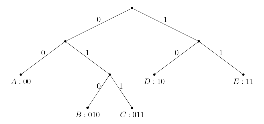
We also notice that a binary prefix code is uniquely defined by a binary tree:

where the root-to-symbol path determines the codeword, and symbols are always leaves. Convince yourself that any construction like this results in a prefix code.

We will now show that the expected codeword length $L$ of any prefix code over $\mathcal{X}$ is bounded by

where $X$ a random variable that takes on values from the set $\mathcal{X}$ with probabilities $(p_1,\dots ,p_n)$. Most importantly, we see that the entropy of $X$ is a lower bound for how much a distribution can be compressed, or equivalently, how much information it contains.

Kraft’s Inequality

Suppose that $l_i$ is the length of the $i$th codeword. If the code is prefix-free:

Proof:

Let $l_{\text{max}}$ be the length of the longest codeword. We notice that:

1. There are at most $2^{l_{\text{max}}}$ nodes at level $l_{\text{max}}$
2. For any codeword of length $l_i$, there are $2^{l_{\text{max}}-l_i}$ descendents at level $l_{\text{max}}$.
3. The sets of descendents of each codeword are disjoint (since one codeword is never a descendent of another)

These imply

Why $\le$ instead of equality? Because it is possible that a node at level $l_{\text{max}}$ is not a descendent of any codeword (consider the tree of the code $\{10,11\}$)!

Lower bound for L

Now, let’s consider the expected codeword length

We will show that entropy is a lower bound for $L$, or

Proof:

Where the final inequality is due to 1) KL divergence being non-negative and 2) to $c\le 1$ due to Kraft’s inequality. One thing to note is that if $l_i=-\log p_i$, $L=H(X)$, the theoretical minimum. The reason we cannot always achieve this is because $-\log p_i$ need not be an integer, which is obviously required.

An Upper Bound for L

Notice that it is possible to construct a prefix code with lengths

since they satisfy Kraft’s Inequality:

By the definition of the ceiling function

Taking the expectation over $p$, we get

This shows that $H(X)+1$ is a good upper bound for L!

In summary, entropy is a lower bound, and a reasonable estimate, for the average number of bits it takes to encode a distribution as a prefix code.

References

• Alon Orlitsky’s ECE 255A Lectures, UCSD
• Cover, T. M., & Thomas, J. A. (2006). Elements of Information Theory. Wiley-Interscience.